SAMPLE
Shadow Autozygosity MaPping by Linkage Exclusion
This program is designed to run on Windows XP SP3 or Vista SP1 systems that
have the .NET 2.0 framework installed, which is freely available from Microsoft
.
Genotyping should be performed using very high density SNP microarrays such
as Affymetrix SNP5 or SNP6 chips. SNP6 data files must be annotated with
chromosome and positional data, which can conveniently be done using SNP6Annotator.
Assumptions and DNA availability
The underlying algorithm of SAMPLE works on the
following assumptions about the families and disease gene:
- The disease is a recessive condition.
- The affected indiv iduals all have mutations in the same gene.
- The families are inbred and the pathogenic mutation is inherited identical
by descent (IBD) in affected indiv iduals.
- Only one mutant allele is present in each pedigree (although each pedigree
may have a different mutation).
The program was specifically designed for instances where it is not possible
to obtain DNA suitable for microarray SNP analysis from affected indiv iduals,
while it is still possible to analyse their parents and unaffected siblings.
Data entry
Adding parents
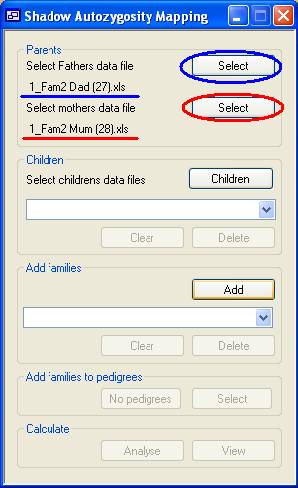
Figure 1 Each family is added sequentially and must include both parents. (Children
are optional.) A parent is added by using the appropriate Select button (Figure 1, highlighted in blue for a father
and red for a mother) to load the parent's SNP data file. The name of the file
will then be displayed by the program (red and blue underlining in Figure
1).
Adding unaffected sibs of affected patients
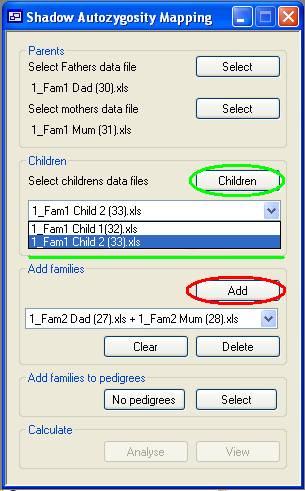
Figure 2 A family may optionally also include one or more children, whose data are
added using the Children button (highlighted in green
in Figure 2). The name of the selected data file will be added to the drop-down
list (green underlining in Figure 2). To remove a child, select his or her file
from this list box and press the Delete button. To
remove all children, press the Clear button which is
also located under the drop-down list of children's filenames.
Adding a family
Once the parents and children have been added, the family can be stored by
pressing the Add button (highlighted in red in Figure
2). This clears the display of the names of the files linked to the family, and
instead adds a family name entry to the second drop-down list, below the Add button. This family name is created by combining the
father's and mother's file names. Families can be removed from the analysis
using the additional Clear and Delete buttons below the drop-down list of family names.
Adding families to pedigrees
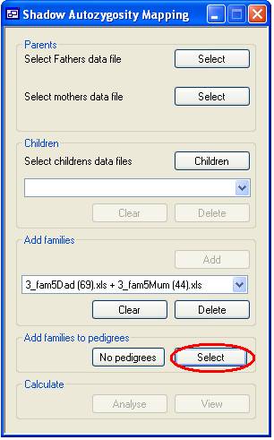
Figure 3 Once all the families have been added, related nuclear families may be linked
to an extended pedigree by pressing the Select button
(Figure 3, highlighted in red). (Alternativel, if there is no known kinship
between any of the nuclear families, this must be specified by clicking No pedigrees.) After clicking Select, the form shown in Figure 4 will be displayed, in
which the families are listed in the upper and pedigrees in the lower drop-down
list box.
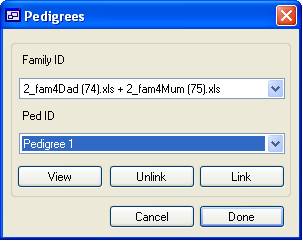
Figure 4 Initially the pedigree list only contains one entry, but once a family has
been linked to this pedigree, a new, empty pedigree will be added to the end of
the list. To link a family to a pedigree, select the family from the upper
drop-down list and the pedigree from the lower list, and then press Link. A family can only belong to one pedigree; thus, if the
family is linked to a second pedigree, it will be automatically unlinked from
its previous pedigree. To unlink a family manually, select it from the upper
list and press Unlink. It is assumed that families
that are not linked to any pedigree are not related to one another. It is
therefore not necessary to create pedigrees for a single family.
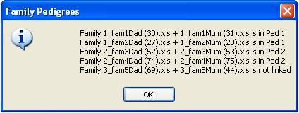
Figure 5 When all pedigrees have been specified, press the View button to display an information window listing the
families and the pedigree to which each is linked (Figure 5). If this is
correct, press the Done button at the bottom of the
previous form (Figure 4).
Viewing the analysis results
Analysing and viewing the data
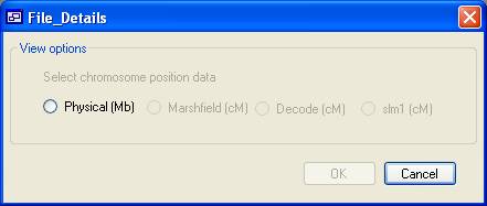
Figure 6 To analyse the SNP genotype data, click Analyse at
the bottom of the main form and choose the unit of distance you wish to use
(Figure 6). Only distance units present in the data file of the father in the
first family can be selected; e.g., in Figure 6 only physical distance is
enabled, since the file contains no genetic map data.
The program will then load the data, first checking for SNPs that have either
a Nocall genotype or show non-Mendelian inheritance;
such SNPs are discarded from the database and any subsequent analysis. Pressing
the View button next to the Analyse button now opens a new window displaying the results
of the analysis (Figure 7).
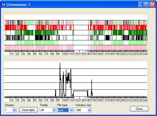
Figure 7 As with IBDfinder and AutoSNPa, the results are displayed
visually and no mathematical or statistical analysis is performed. Rather, the
program highlights the movement of large segments of the genome from parent to
child, which have undergone relatively few recombination events. The sizes of
the fragments that contain the mutant allele are very variable, and the length
of a common region consequently does not predict whether or not it contains the
disease gene.
The results window displays the data one chromosome at a time, with Chr. 1
initially selected (Figure 7). The window contains two display panels; the upper
panel shows the positions of SNP that exclude linkage to a disease gene, while
the lower panel shows a graph of an empirically derived score, plotted against
chromosomal position.
Features common to both panels
Both panels are drawn to the same scale, indicated by the rulers at the
bottoms of the panels. The units are Mb or cM according to whether physical or
genetic map position data were selected earlier. Just above the displayed map
positions on the ruler is a discontinuous thick black line, within which the
gaps represent regions of no SNP coverage. Each chromosome is drawn to the same
scale, such that the longest chromosome spans the full panel width.
Upper panel
The upper panel is composed of six strips of vertical markers. Each marker
represents a SNP that can be excluded from linkage to the disease gene. Thus,
the absence of markers suggests a region may be linked to the disease locus. The
colour of each marker represents the reason the SNP was excluded, as
follows:
| Red: |
SNPs for which the parents within one nuclear family are homozygous
for different alleles. |
| Dark green: |
SNPs for which unaffected children within a single nuclear family are
homozygous for both alleles. |
| Black: |
SNPs excluded because a child whose parents are heterozygous is
homozygous for the same allele as another parent within the same
pedigree. |
| Pale green: |
SNPs excluded because unaffected children of heterozygous parents
within a pedigree are homozygous for both alleles. |
| Pink: |
SNPs excluded because the parents within one pedigree do not share a
common allele. |
Each strip displays SNPs excluded on one of these five criteria, except for
the uppermost strip, which shows combined information for all the excluded SNPs.
Lower Panel
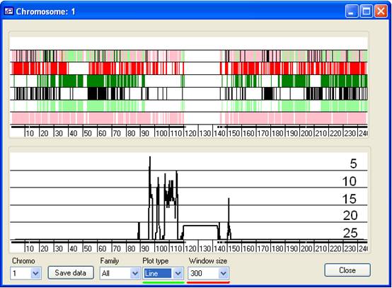
Figure 8 Due to the limited screen resolution, compared to the large number of SNPs
per chromosome, multiple SNPs are likely to occupy the same pixel on the screen.
It is consequently difficult to discern whether a region has been excluded by
just a few or by many SNPs. To give an indication of the number of SNPs that
exclude a region, the lower panel shows a graph of the number of non-excluding
SNPs in a sliding SNP window. The size of this window is set using the Window size drop-down list box (Figure 8, underlined in
red). Since most SNPs are uninformative, the graph only shows regions that have
25 or fewer excluding SNPs. The horizontal gridlines indicate the number of
excluding SNPs in the window and are labelled in Figure 8.
A 
B 
Figure 9
Initially, this value is plotted as a line graph, with the points indicating
the centre of the SNP window. However, since SNP density is not uniform along
the chromosome, it is alternatively possible to view the graph as a series of
tapes or bars that show the extents of the windows (Figures 9A,B). While the
Bar view displays the width of a window, it is
possible for regions to overlap, making them appear to be one wide region. To
overcome this, the Tape plot highlights points where
regions overlap. These different plots are selected using the Plot type drop-down menu (underlined in green in Figure
8).
View options
Below the lower results panel is a series of controls for changing the view
options of the two panels. These include the Window size and Plot type controls described above, while the others
are used respectively to select the chromosome displayed, select information
from a single family and save the underlying data to a file.
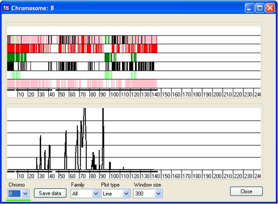
Figure 10
- Chromo list:
- This contains a list of the autosomes, used to select which chromosome is
displayed. (The current chromosome is also indicated at the left-hand side of
the title bar.) For example, to view Chr. 8, select 8 from the list (Figure 10, green underlining).
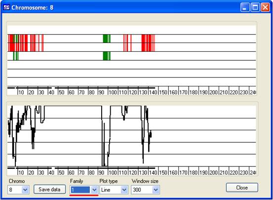
Figure 11
- Family list:
- By default the All value is selected and data
from all the families are shown in the panels. To view regions excluded by a
single family, select the number from the list, representing the order in
which that family was added. For example, to view data for the first family
added to the program, select 1 (Figure 11,
underlined in red). Note that since only data from a single nuclear family are
now shown, SNPs are no longer excluded by analysis across a pedigree.
Therefore, only red and dark green marks appear in the upper panel.
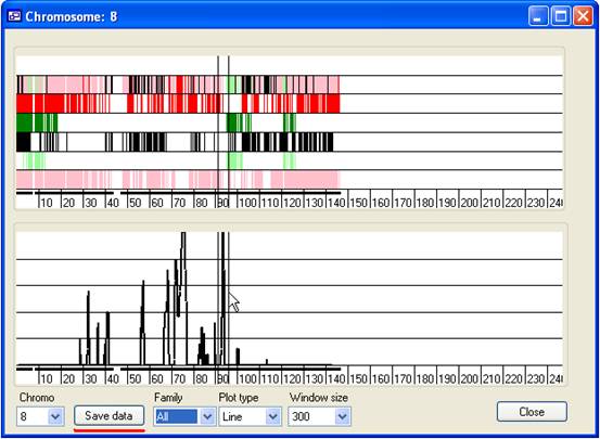
Figure 12
- Save data:
- A region's underlying data can be exported either to a colour-coded web
page or to a tab-delimited text file. To select a region, place the mouse
cursor at the start of the region (on either the upper or lower panel) and
while holding down the left mouse button, drag the cursor to the end of the
region. The currently selected region will be delimited by two black vertical
lines on the upper and lower panels (Figure 12). To save the data, press Save data (underlined in red in Figure 12) and enter
the name of the output file and the desired file extension.
- Window size:
- The lower panel represents a graph of the number of non-excluding SNPs in
a sliding window. This value can be set to 100, 200, 300 or 400 SNPs (Figure
13A-D, respectively).
Interpreting the results
The SAMPLE algorithm works by tracking the movement of large segments of
chromosomes from parents to offspring. Each family has rather little information
content, compared to standard autozygosity mapping. The discriminative power
derives from collating the exclusion information across a number of families.
The size of a region therefore depends on the unpredictable way in which the
regions from each family overlap. As in classical autozygosity mapping,
therefore, the disease gene may fall in a very large region or a very small one
that does not stand out from the background noise.
In the data shown above, the disease gene is located at 94.7 Mb on Chr. 8.
The peak in the graph corresponding to this position is the third largest at a
window size of 300 SNPs. However, at 400 SNPs the peak almost disappears, and is
approximately the 15th ranking peak. At 200 SNPs, the peak is still one of the
more prominent peaks, but the difference between it and other similar peaks is
not as clear as at 300 SNPs. Therefore, the SAMPLE program should ideally be
used to screen a list of candidate genes or regions that have been identified by
other means.
|